Considerations For Accelerating On-Device Stable Diffusion Models

One of the more powerful – and visually stunning – advances in generative AI has been the development of Stable Diffusion models. These models are used for image generation, image denoising, inpainting (reconstructing missing regions in an image), outpainting (generating new pixels that seamlessly extend an image’s existing bounds), and bit diffusion.

Stable Diffusion uses a type of diffusion model (DM) called a latent diffusion model (LDM) developed by the CompVis group at LMU Munich. Much of its appeal is that it is entirely open-source and is publicly available for anyone to use. Currently, it is used for image synthesis, text generation, and anomaly detection in art, natural language processing, and cybersecurity applications. For example, game developers can use it to generate characters and game scenes from text descriptions.

Diffusion models train by adding noise to images, which the model then learns how to remove. The model then applies this denoising process to random seeds to generate realistic images. However, due to the complex computation process, including a mix of matrix and vector operations, image generation speed can become a bottleneck. Deploying these models—which can have over 1 billion parameters—on-device can be challenging due to restricted device computational and memory resources. The ideal solution is a neural network accelerator that supports convolution and attention-based models. Still, there are ways to accelerate generative AI on existing hardware, which we explore in the following discussion.

Model architecture

Stable Diffusion uses a variational autoencoder (VAE) to generate detailed images from a caption with only a few words. Unlike prior autoencoder-based diffusion models, Stable Diffusion incorporates a U-Net backbone with cross-attention layers to reduce noise while learning the latent representation. This enables the model – or, more precisely, sequence of models – to learn (often uncannily) photorealistic images with fewer compute resources.

Fig. 1: Examples of images generated from text using Stable Diffusion. Source: https://github.com/CompVis/stable-diffusion/

While efficient, Stable Diffusion comprises about one billion parameters between the constituent encoder, U-Net, and decoder models. A text encoder with an input sequence length of 77 and an output embedding size of 768 adds about 85 million parameters to the model pipeline. Deploying Stable Diffusion in resource-constrained environments thus requires hardware and software optimizations and support for numerous matrix and vector operations.

Like other state-of-the-art models for extracting information from text and generating images, most Stable Diffusion operations (98% of the autoencoder and text encoder models and 84% of the U-Net) are convolutions. The bulk of the remaining U-Net operations (16%) are dense matrix multiplications due to the self-attention blocks. Convolutional and batch matrix multiplication layers comprise over 99.9% of the four models in the Stable Diffusion pipeline.

However, most of the layers in these models are neither convolutions nor dense matrix multiplications. Each model contains numerous vector arithmetic operations: addition, constant multiplication, division, and (in the autoencoder) subtraction, plus mean, reshape, transpose, and other layers. Processing these layers and optimally managing the reading and writing of activations is a challenge for deep learning accelerators.

Different releases of Stable Diffusion support different image resolutions. The first major version of Stable Diffusion produced 512×512 RGB images. Stable Diffusion 2 uses 768×768 images, and Stable Diffusion XL was trained on 1024×1024 images.

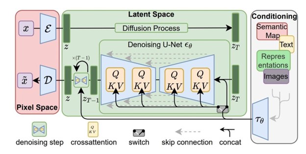
Fig. 2: Stable Diffusion model architecture. Source: https://scholar.harvard.edu/binxuw/classes/machine-learning-scratch/materials/stable-diffusion-scratch

The text encoder model takes an input sequence (of length 77 in the initial model), learns a hidden state for each element in the series, and outputs encodings of a given size. For an implementation with an output size of 768, a simplified ONNX representation of the model contains 84.9 million parameters and 13.3 billion operations. Implementing the model with 8 MB SRAM has many weights (85.9 million weight moves) relative to activations (a working buffer of 11.0 million bytes). Unless available weight memory is comparably high relative to activation memory, the partitioning of the text encoder will be constrained by the volume of weights rather than activations.

The VAE is symmetric: the encoder’s input size matches the decoder’s output size and vice versa. However, the decoder contains twice the operations and approximately 45% more parameters than the encoder model, most of which are in the convolutional layers. Unlike the text encoder, the VAE is activation-heavy. Using the same 8 MB cut, an encoder with a 512x512x3 input and a 64x64x3 output contains a working buffer of 78 million bytes and 1.7 billion activation moves (to and from external memory) but only 34.1 million parameters.

The design of the initial convolutional layer – which generates 128 channels while retaining the 512×512 input shape – is responsible for many activations. After the initial convolutional layer, the network holds this 32 MB output in memory while applying the following operations: two subsequent convolutions, instance normalizations (which involve flattening the height and width, normalizing, and then reshaping the output back to four dimensions), constant add and multiply operations, and sigmoid activation functions. However, it is possible to recompute these skip connections, computing the initial convolution twice rather than holding it in memory, reducing activations while increasing weights. This optimization may lead to more efficient model partitioning, decreasing the total activation moves and increasing model throughput.

The decoder portion of the VAE contains even more activations: a working buffer of 133 million bytes and 3.6 billion activation moves to go along with 49.5 million parameters. The decoder starts with a smaller input volume (64x64x4). Still, it generates a large volume of activations like the encoder, this time with a convolutional layer that increases the output shape to 512x4x3x3. As with the encoder, the decoder holds this large activation volume in memory while computing two additional convolutions, constant multiplications and additions, layer normalization with reshaped inputs and outputs, and sigmoid activations.

Most of the operations and parameters in the stable diffusion pipeline are in the U-Net denoising model. The input and output to the U-Net is the 64x64x4 output from the encoder, which is then passed as input to the decoder. This U-Net has 865 million parameters and over 1.6 trillion operations and contains large activations in the attention blocks. One of the batch matrix multiplication operations alone generates an output volume of 160 MB.

The presence of large skip connections also allows for the optimization of activations by recomputing inputs. Unlike the autoencoder, where most compute cycles are matrix multiplications (including convolutions), the U-Net has many vector operations in the attention blocks. To support this U-Net – and Stable Diffusion – a processor needs to be able to run a mix of quantized and floating-point arithmetic and reshaping operations.

Hardware acceleration

In the future, hardware accelerators for neural networks will need to support attention-based models for processing text and, increasingly, for vision applications. Stable Diffusion contains elements of several architectures, coupling a variational autoencoder with a backbone network that uses convolutions and cross-attention blocks to extract information in the latent space. For an AI model developer to run Stable Diffusion effectively, hardware and software must efficiently execute each architecture’s operations.

For an architect designing a neural processing unit, floating point, quantized operator support, and model performance are priorities. A chip must be able to run Stable Diffusion and related models at sufficiently high throughput and low latency without a decline in accuracy. This could be especially challenging for certain edge processors with limited power and area.

Stable Diffusion is thus a critical test for an artificial intelligence processor. It demands that the processor support a range of matrix and vector operations. It requires the processor to handle diverse models and blocks of models: some comprised primarily of weights, others of activations. And with the state of the art in generative AI advancing rapidly, future models will likely become more complex.