EM Analysis At Advanced Nodes

EM statistics
Almost 50 years ago, James Black demonstrated experimentally that TTF of the metal line stressed by direct current (DC) of density j at the temperature T follows the dependency

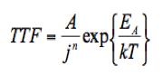
where k is the Boltzmann constant, and A is the proportionality coefficient, which can depend on line geometry, residual stress, and temperature. Two critical parameters, the current density exponent n and activation energy are the subjects of extraction from the measured TTF. To estimate when the failure will happen in a real-time interval of several hours, these measurements are carried out at the so-called stressed conditions, characterized by elevated temperatures of 200 – 400oC and high current densities of 3×10(9) – 5×10(10) A/m(2). TTF is measured in test structures consisting of hundreds of identical lines loaded with the same currents, and MTTF is extracted from the accumulated TTF measurements. Failure times are customarily fitted to the lognormal distribution

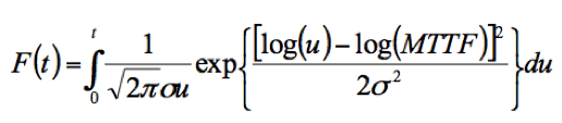
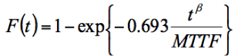
where F(t) is the cumulative percent of failures at time t, and  is the standard deviation. A better fit to the measured TTF in metal lines with different lengths is achieved by using the Weibull distribution

Both MTTF and are found by plotting the experimental TTF data in a lognormal plot; the coefficient is extracted from Weibull plot. All of these parameters are extracted from measurements taken against a variety of test structures designed for different metal layers and different current directions (upstream and downstream tests), as shown in Figure 5.

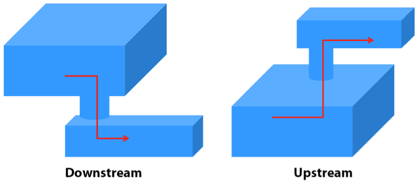
Figure 5. Downstream and upstream EM test structures. Red arrows are the electron flow directions.

Current EM assessment methodology
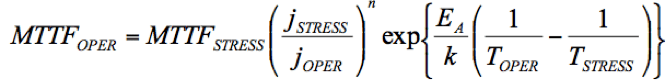
In current EM analysis methodology, prediction of MTTF at operating conditions (characterized by lower temperatures and current densities) is based on measured MTTF at stress conditions, using the equation

Knowing MTTF and the failure probabilities for each type of interconnect segments and all metal layers allows engineers to calculate failure times for every segment with different geometries, using the independent element model.

However, not every segment of the chip metallization requires calculation of MTTF. As previously discussed, the EM-induced development of the critical level of stress is required for damage initiation. On the other hand, continual stress build-up generates an increase in stress gradient, which is responsible for the atom backflow directed toward the cathode end of the line (atoms diffuse from the areas with compressive stress toward the areas with tensile stress). The shorter the line, the larger the stress gradient that is generated by the same build-up stress, which leads to larger atomic flux flows toward the cathode. A steady state is developed when the EM-induced atomic flux is balanced by the stress gradient-induced backflow of atoms. This steady state is characterized by a linear distribution of the hydrostatic stress along the line, which remains steady unless the electrical load is changed. If the maximum value of the tensile/compressive stress is less than critical, void/hillock formation will not occur. Any such segment is deemed “immortal,” and should be filtered out of the pool of analyzed segments.

This filtration consists of first calculating the product of the electrical current density j and the metal line length l for each segment, and then comparing calculated products with the so-called Blech critical product:

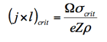
which states that any segment characterized by a smaller current-length product than a critical one will be immune to EM failure. Here, is the atomic volume; e is the electron charge, eZ is the effective charge of the migrating atoms, p is the wire electrical resistivity, and  is the critical stress needed for the failure nucleation (void/hillock). After removing all immortal segments, the MTTF is calculated for the remaining segments. When the failure probability of i-th element Fi(t) is known, the chip level failure probability, Fchip(t), can be calculated, based on the weakest link statistics

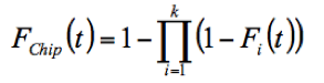
where k is the total number of elements with EM concerns in a chip.
Thus, the simplest methodology for EM assessment in Cu interconnects consists of:

1. Extraction of interconnect segments from layout;
2. Estimation of the current density, j(i) in each segment;
3. Filtration and removal of the immortal interconnect segments using immortality criterion;
4. Calculation of the failure probability for each remaining interconnect segment, and
5. Calculation of the full chip failure probability and MTTF.

EM-induced failure rates of the individual segments are considered as a measure of EM-induced reliability, and the MTTF of the weakest segment is accepted as a measure for the chip lifetime. This methodology provides a very conservative estimate of the top limit for the current density that can be used in a particular technology node to avoid EM failure.

To view part one of this series, click here.
To view part three of this series, click here.