There’s More To Machine Learning Than CNNs

Neural networks – and convolutional neural networks (CNNs) in particular – have received an abundance of attention over the last few years, but they’re not the only useful machine-learning structures.

There are numerous other ways for machines to learn how to solve problems, and there is room for alternative machine-learning structures.

“Neural networks can do all this really complex pattern recognition stuff, especially the convolutional neural networks,” said Elias Fallon, software engineering group director, custom IC & PCB group at Cadence. “Their downside is that they’re so big, and they require tremendous amounts of data in order to train them.”

Some structures, like decision trees, are as old as neural nets in concept, but they aren’t neural networks. Others leverage more common neural-net structures in new ways. We’ll walk through some of them here to understand what they are and what they’re good for, starting with what’s more familiar to establish a baseline.

Conventional neural networks
Artificial neural networks (ANNs), the most familiar structures, deepen the original perceptron idea. They provide many layers that first identify important features in the data being fed to them, and then they do something useful with that information, such as classifying images or translating languages.

Convolutional neural networks (CNNs) arguably have the most dedicated hardware solutions. They can be enormous – and they’re getting bigger. They’re good at making inferences based on visual data – still images and video.

Also well-known are recurrent neural networks (RNNs), which are a generic class of structure distinguished by their ability to deal with time-series or sequential data. That means that they need to keep some data around, since early data may inform decisions on later data. So while CNNs are feed-forward only, RNNs have layers where they may store data for future use or even feed it back to earlier layers.

With plain RNNs, the memory of past events fades pretty quickly. LSTMs – long short-term memory units – are a type of RNN with memory for holding onto past events for a longer period of time. Related to that are gated recurrent units (GRUs), which do what LSTMs do in a somewhat simpler manner.

RNNs, by nature, look at data as it appears in order. There is another approach that we’ll look at, however, that’s proven more effective than the basic RNN, and it’s getting traction.

As compared to some of the other structures we’ll discuss, ANNs are better at so-called knowledge transfer. “You train on certain samples, and, once you get brand new samples, you can pick up where you left off,” said Venki Venkatesh, director of R&D for AI & ML solutions in Synopsys’ Digital Design Group. Some of the other approaches require complete retraining if new data is added.

ANNs excel at pattern recognition – whether visual or audio. And they’re huge. “The models are really big, measured in terms of the number of coefficients,” said Fallon. “But that lets them do all these things that are not obvious to us humans.”

If a linear or polynomial curve fit can be thought of as the simplest possible decision engine, then ANNs are the most complex. Some of the following structures lie somewhere in the middle.

Decision trees
A decision tree is just what it sounds like: a simple tree where, at each node, a decision is made, and inference travels down the path according to that decision. Exactly what that decision is will be partly affected by the developer and partly by the training.

Fig. 1: A simple decision-tree example. Source: Wikipedia

Unlike conventional neural nets, decision trees don’t extract features from the data. So-called “feature engineering” is done by the development team. “CNNs naturally do that feature engineering,” said Cadence’s Fallon. “Decision trees don’t have that ability.”

Others agree. “Decision trees and other similar structures usually take fewer inputs, not a whole image as input,” said Michael Kotelyanski, senior member of technical staff at Onto Innovation. “Some feature engineering is required to convert input image into a lower-dimensional input vector for them. But the inference and training may be less computationally intensive.”

Given those features, the developer specifies how many layers deep the decision should be, and then the training decides which features are used for which stage of the tree, as well as what the specific decisions will be.

“It goes through the same kind of training process we think about with neural networks, but not with a neural network structure,” said Fallon. “It’s this tree structure and deciding which variable and what value I use.”

Consider a digital game of 20 questions. Each question leads the inference in a particular direction. They’re often used where heuristics might have been used in a pre-machine-learning approach. In fact, those heuristics might have been layered in trees, as well. The difference is that in the older case, the decisions were specifically created by the developer, while the machine learns the heuristics in a decision tree.

Decision trees are more accessible to humans than ANNs. It’s easier to examine a tree and understand the decisions at each point than it is to make sense of the weights and connections in an ANN.

This can be helpful when the training data is sensitive and proprietary, since it’s easier for non-expert in-house developers to train without involving anyone else. “Decision trees are more accessible to most of us,” explained Fallon. “You don’t need a team of experts to get them to train correctly. We have to have the simpler models that are a little more reliable, because they have to be able to train on the customer data at the customer site.”

As one example, EDA tools may use decision trees when trying to optimize layouts or identify possible yield limiters in a layout. “When we use them in our software flows, what we’re replacing is the heuristics,” said Fallon. For example, “We look at analog schematics and say, ‘Which transistors should be grouped together? Are they connected to the same nets? Do they have the same width? Do they have the same length? Are they the same size, but the same type?’”

Random forests
Random forests take decision trees one step further. In order to improve the reliability of the decisions made, random forests involve many decision trees, effectively crowdsourcing the answer by averaging or combining the results of the different trees.

Fig. 2: A random forest consisting of multiple decision trees trained on different subsets of the training data. Results of each tree are combined or averaged. Source: Venkata Jagannath, CC BY-SA 4.0

“The way they work is that you’ll put in, say, 100 trees and then take 100 random different subsets of the training data,” said Fallon. “Each tree is trained on a different subset of the data. On average, they do a much better job of coming up with the right answer than giving one tree all the data.”

So if a decision tree is like 20 questions, then a random forest is like 100 people independently playing the same 20 questions and then combining the results. Or maybe it’s more like Family Feud, where “survey says”…

Random forests may work hand-in-hand with ANNs as triage classifiers. “Decision trees, random forests, and other like classifiers can act to reduce load and discrepancy on the deep-learning classifier,” said Mike McIntyre, director of software product management at Onto Innovation, describing use when visually inspecting for defects as an example. “The first-order classifier is able to work with a few descriptors, such as size, shape, color, background, and position and pre-classify the defects to a relatively high level (70% to 80+%). The defects with low confidence or unknown classification, or those deemed important enough, get fed into the secondary ANN classifier, which is more expensive to run.”

Boosted trees, or gradient-boosting machines
Boosted trees resemble random forests in that they involve a collection of decision trees. But rather than creating all of the trees independently and then combining their outputs at the very end, the trees are built – and calculated – sequentially.

The first tree might be a so-called “weak learner.” So a second tree is built that improves the learning from weakly correlated training points. And then a third tree is built that improves on the second. In other words, unlike random forests, the trees are not uncorrelated. They are derived from each other.

Some feel that boosted trees can do a better job, on average, than random forests – unless your training data is noisy, which may result in overfitting. “I have known some applications where boosted trees are performing far better than the neural nets,” said Venkatesh.

Generative adversarial networks, or GANs
To understand GANs better, it’s helpful to break them into two separate notions.

The first is the “generative” part. If you think of a classic CNN, it takes a ton of data – the pixels in an image – and by identifying features, it abstracts the content down into smaller and smaller layers. Some think of this as a form of compression, because in theory the compressed version still contains all of the information in the original image, just expressed more concisely. So you should be able to take that compressed version and decompress it — that is, take it through a reverse network that eventually expands it into the original image. That reverse process could be used to generate an image from some distribution function.

The second notion is the “adversarial” aspect. We bring in two networks, one a generator (of images, perhaps), and the other a “discriminator” that evaluates the generated image or some other artifact. The discriminator will have previously been trained to recognize whatever it is the generator is going to put out. The GAN training involves the generator creating images and then having the discriminator decide whether it sees them as “real” or not.

“It’s basically taking two CNNs and pitting them against each other,” said Ron Lowman, strategic marketing manager, IP at Synopsys.

Keith Schaub, vice president of technology and strategy at Advantest, explains this concept further. “For the basic classification problem (e.g., “Is it a hot dog?”), one algorithm generates fake hot dog images, while the other one guesses if the image is fake or not. This back and forth continues until an equilibrium is reached, whereby the ‘faker’ will be generating amazingly life-like images, sounds, voices, or whatever the classification is.”

Fig. 3: Basic GAN architecture. The generator creates an image from a random seed. The discriminator evaluates the image based on its training to see if it can tell real from fake. The result goes back to the generator and discriminator so that they improve. Source: Bryon Moyer/Semiconductor Engineering

As an example, the discriminator may have access to samples of artwork created by Van Gogh. The generator then creates images, and the discriminator decides whether or not they were created by Van Gogh. If not, then both the generator and discriminator are updated. This feedback acts as training for the generator to create better images, and for the discriminator to do a better job of adjudicating. Eventually, the generator will learn to create images that fool the discriminator. That point is reached when the discriminator says there’s a 50-50 chance of the image (or whatever artifact was created) being real vs. fake.

GANs are what allow algorithms to take a picture of your face and figure out what you might look like in 10 years, for example. Or it might help to tell what you might look like in a new outfit, or with different hair, or with someone else’s face.

On the more questionable side, they also help to create fakes and deep fakes that are incredibly hard, if not impossible, to tell from true images or videos. “There’s this application where they used samples of a few celebrities,” related Venkatesh. “And then they created images of faces – all artificially created. But they looked so real you would not be able to find out that this is an artificially generated face.”

Transformers
This is a structure that has changed how sequential input is processed. While RNNs take the data in order, transformers can evaluate data out of order. It’s gotten a lot of traction with natural language processing (NLP). In that context, rather than scanning a sentence from beginning to end, you can process the entire sentence at once.

“New techniques like transformers are coming down the road that will hopefully replace LSTM’s and RNNs,” noted Gordon Cooper, product marketing manager for ARC EV processors at Synopsys.

This helps processing speed, since you can run different parts of the sentence in parallel. It’s been used to great effect in the BERT series of networks for language translation, but it’s also being evaluated for object classification as well.

One of the concepts that transformers leverage is referred to as “attention.” It focuses analysis on what appear to be more salient parts of the network for a given set of data being inferred. Larger numbers in vectors or matrices are what focus the attention of the engine.

These algorithms may involve multiple passes, but because they can handle an entire sentence at once, they can correctly reorder words as appropriate for a different language. If the sentence was processed one word at a time, the resulting construct would sound more stilted and not at all natural. Alternatively, a separate reordering step might be necessary.

Support vector machines, or SVMs
The original two-dimensional classification problem can be simplistically described as finding a line or curve that cleanly separates a set of data into two parts, each of which is in a different class.

But what if the data is intermixed? Then there’s no way to identify a dividing line or curve – at least not in two dimensions. What support vector machines do is promote the dimensionality of the problem repeatedly until a clean divide, referred to as a “hyperplane, ”can be found. While accurate, training is slow, so they’re better for small, clean data sets.

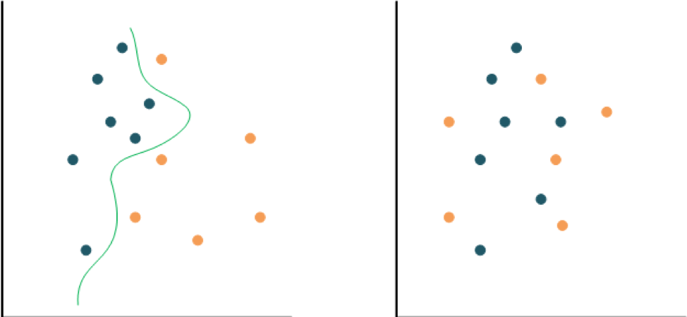
Fig. 4: On the left, a curve can be fit between the two sets of points in order to classify them. On the right, that’s not possible (within reason), so an SVM will play with dimensionality to make such a split possible. For instance, if the right one had a third dimension representing the height above the page, it might turn out that all the orange nodes are above the blue ones, making a clear separation easy. Source: Bryon Moyer/Semiconductor Engineering

Graph neural networks, or GNNs
GNNs help with graph analysis. For example, given a graph with some labeled nodes, a GNN will attempt to label the unlabeled nodes.

Social media graphs are a good example, where each node represents a user and the edges represent connections. The graph can be manipulated to cluster nodes based on feature similarity, classify the nodes, predict connections where there are none yet, and many other operations.

A large number of phenomena can be illustrated with graphs, so there are many applications for which GNNs can be helpful , including ones that other networks can work on, such as images and language. But it goes far beyond that. For example, molecules can be represented as a graph of atoms and bonds.

Some GNNs can learn dynamically, like CNNs can, when the graph changes. Others require complete retraining when new nodes are added to the graph.

Graph convolutional networks, or GCNs
GCNs could possibly be thought of as a cross between a type of GNN and a CNN. If you think of an image as a two-dimensional graph of pixels, then a CNN is well suited to work on that graph. But it doesn’t work so well for more general graphs.

That’s what GCNs work on. They do a similar job of aggregating nodes and their neighbors, but the kernels or filters don’t all have to be the same for each node. You can think of it as a generalized CNN, although the math is different. Likewise, some refer to a CNN as a specific GCN.

That said, GCNs are newer than CNNs and are an area of active research.

Graph-matching networks, or GMNs
Graph-matching networks are used to evaluate the similarity between different graphs. Rather than taking two graphs, running computations on each, and then comparing results, GMNs work on the two graphs in bare form, finding, for example, similar nodes within the graphs before doing the computations. It uses what’s referred to as cross-graph attention to focus on key nodes.

Generative matching networks, or GMNs
Yes, this is a GMN that is completely different from the prior GMN.

Generative matching networks create samples according to a distribution. In fact, this is another, more direct way of doing what a GAN does. Effectively, they create one graph and then compare it to a reference graph, ultimately trying to reduce the comparison errors over many iterations.

GMNs are conceptually simpler than GANs, but in practice, the calculations required to compare the generated and reference graphs are arduous. “GMNs requires two probability functions (the ‘true’ one and the ‘generated’ one) to be compared based on samples,” said Venkatesh. “This is hard to do. Practically, they are not easy to set up and train.”

So, while GANs might seem like a more indirect way of doing things, they are used far more than GMNs are.

Conclusion
Many of these less common ways of doing inference are still being extensively studied. The ones that are better developed are likely to be more data center-focused than something that would run at the edge. So CNNs and transformer-based networks are more likely to appear at the edge than the others, and they’re also the ones attracting dedicated hardware platforms.

“The state of the art in academia explores lots of stuff, and then the broadest deployment is in the data center,” said Geoff Tate, CEO of Flex Logix, which focuses on edge inference. “Almost everything we see are CNNs of various kinds.”

The networks in earlier research may or may not enter the mainstream, either in the data center or the edge. If any of them achieve the popularity of CNNs, then we may see efforts to tailor hardware for them, as well.

Related
Developers Turn To Analog For Neural Nets
Replacing digital with analog circuits and photonics can improve performance and power, but it’s not that simple.
Compiling And Optimizing Neural Nets
Inferencing with lower power and improved performance.
Neural Networks Without Matrix Math
A different approach to speeding up AI and improving efficiency.
How To Measure ML Model Accuracy
What’s good enough for one application may be insufficient for another.